A Matrix Factorization Model on tensorflow (with Nonlinear Cross Features)
Sat, Nov 18, 20171. Problem Description
We are given a rating matrix $R$ where only a small fraction of the entries are provided; otherwise the rest of them are missing. The task of a Recommender System is to predict those missing entries. As in most Machine Learning problems the assumption here is that there’s an underlying pattern of how users rate movies.
By the nature of the problem, $R$ is a sparse matrix, where the sparsity comes not from zero entries but from empty records. Therefor, we represent the data in the rating matrix $R$ in 3 columns: $i$: user ID , $j$: movie ID and $R_{ij}$: the rating (see Table 1).
Table 1. A conceptual sketch of the Ratings in ml-20m data in sparse format
| $i$: user ID | $j$: movie ID | $R_{ij}$: the rating |
|---|---|---|
| 0 | 14 | 3.5 |
| 0 | 7305 | 4.0 |
| 0 | 16336 | 3.5 |
| . | . | . |
| . | . | . |
| 1 | 52 | 4.0 |
| 1 | 986 | 4.0 |
| 1 | 1455 | 3.5 |
| 1 | 1705 | 5.0 |
| 1 | 5598 | 4.0 |
| . | . | . |
| . | . | . |
| 138493 | 27278 | 5.0 |
2. MovieLens 20M dataset
MovieLens dataset consists of 20,000,263 ratings from 138,493 users on 27,278 movies. Sparsity of the matrix $R$ is $0.5\%$ – i.e. ratings are provided for only $0.5\%$ of all possible user-movie combinations.
All ratings are given in the interval [0.5, 5.0] with increments of 0.5:
{0.5, 1.0, 1.5, 2.0, 2.5, 3.0, 3.5, 4.0, 4.5, 5.0}Since the input data was ordered according to user IDs, it was crucial to shuffle the data before splitting it into training, CV and test sets.
The Input Data is split accordingly:
- $64\%$ – training data,
- $16\%$ – cross validation data,
- $20\%$ – test data.
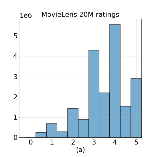
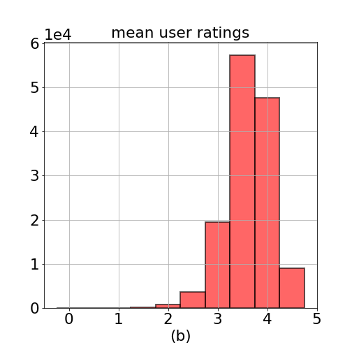
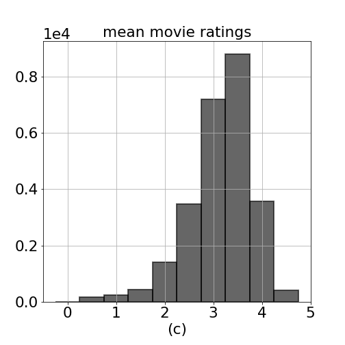
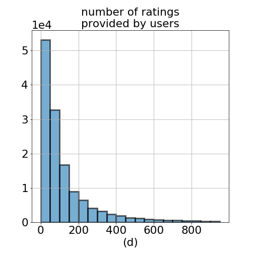
Figure 1. Histogram of (a) all ratings in ml-20m data (b) mean of ratings per user (c) mean of ratings per movie, and (d) number of ratings provided by users. Minimum number of ratings provided by a user is 20, and maximum is 9254 ratings.
3. Matrix Factorization Model
The Collaborative Filtering model used in this problem is based on Matrix Factorization (or Low-Rank Matrix Factorization – which is only another name that refers to the same model). In essence, this model takes only the past ratings as input to the model. That is, no user profile information nor any explicitly defined movie features are used to train the model. The assumption here is that the users who liked the same movies are also likely to favor other but similar movies.
The term collaborative refers to the observation that when a large set of users are involved in rating the movies, these users effectively collaborate to help the model better predict the movie ratings for everyone because every new rating will help the algorithm learn better features for the complete user-movie system.
The Collaborative Filtering Model can also be described as reconstructing a low rank approximation of the matrix $R$ via its Singular Value Decomposition $R = U \cdot \Sigma \cdot V^T$. The low-rank reconstruction is achieved by only retaining the largest $k$ singular values, $R_k = U \cdot \Sigma_k \cdot V^T$.
Eckart-Young Theorem states that if $R_k$ is the best rank-$k$ approximation of $R$, then it’s necessary that:
1. $R_k$ minimizes the Frobenius norm $||R - R_k||_F^2$ and
2. $R_k$ can be constructed by retaining only the largest $k$ singular values in the diagonal matrix $\Sigma_k$ of the SVD formulation.
We can further absorb the diagonal matrix $\Sigma_k$ into $U$ and $V$ and express the factorization as a simple matrix multiplication of the feature matrices $U$ and $V$.
$R_{k(m \times n)} = U_{(m \times k)}^\ \cdot V_{(k \times n)}^T$
where,
the parentheses indicate matrix size,
$m$: number of users ($m = 138493$)
$n$: number of movies ($n = 27278$)
$k$: rank hyperparameter ($k \approx 10$).
$U$: users feature matrix
$V$: movies feature matrix
Hence, we can formulate the problem as an optimization problem minimizing the following loss function $L$ via SGD.
$$argmin_{\ U,V}\ L = ||R - R_{k}||_F^2$$
It’s important to note that the Frobenius norm is computed only as a partial summation over the entries in $R$ wherever a rating is provided—or equivalently over the list of ratings as shown in Table 1. The optimization procedure searches for the values of all entries in $U$ and $V$. There are $(m+n) \times k$ many such tunable variables.
N.B.: We abstain from imposing an explicit bias term in the feature vectors $U$ and $V$. In the Matrix Factorization scheme, the embeddings are free to learn biases if necessary.
The hyperparameter $k$ is to be chosen by cross-validation. Too small a $k$ value would not be enough to explain the pattern in the data adequately (underfitting), and too large a $k$ value would result in a model that fits on the random noise over the pattern (overfitting).
It’s worth to make a brief interpretation of the feature matrices $U$ and $V$. In the $k$-rank approximation scheme, each rating $R_{ij}$ is expressed as the dot product $U_i^\ \cdot V_j^T$ as shown in Figure 2. The goal of our optimization routine is for the model to learn a separate latent feature vector (or alternatively an embedding vector) for each user and movie. The term latent implies that the features are not explicitly defined as a part of the model nor can they be interpreted definitively once the embeddings are learned. Each entry in $U_i$ and $V_j$ corresponds to the weight coefficient of an abstract feature. These features may specify the genre of the movie, the class of actors in it, how much action or drama is contained in the movie or any other distinguishing quality that would help characterize how the users rate movies. Hence, the dot product representation of the ratings $\hat{R}_{ij} = U_i\ \cdot V_j^T$ expresses a linear combination of
1. how strongly that specific feature is favored by the user-$i$, and
2. how much that specific feature is contained in the movie-$j$.
The terms $R_{k}$ and $\hat{R}$ are used interchangeably to refer to the low-rank matrix approximation of the original partially filled rating matrix $R$.
Figure 2. A conceptual sketch of the ratings matrix $R$ decomposed into its factors: user and movie feature matrices, $U$ and $V$. The dots ‘$\cdot$’ in the figure illustrate provided rating values; and question marks ‘$?$’ the missing values. Each entry $R_{ij}$ is expressed as a dot product of the user and movie embedding vectors $U_i$ and $V_j$, respectively.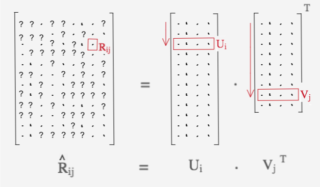
4. Linear, Nonlinear and Cross Features
Linear Terms:
The standard collaborative filtering model consists of only the following linear term: $$\hat{R}_{ij} = (R_{lin})_{ij} = U_{i}^\ \cdot V_{j}^T$$ In this dot product, $p^{th}$ feature coefficient of $U_{i}$ is multiplied with the corresponding $p^{th}$ coefficient of $V_{j}$. The contributions from each feature are added up into a total sum.
Subsequently, I added a sigmoid filter $R_{ij} = 4.5 \cdot \sigma(U_i^\ \cdot V_j^T) + 0.5$ which forced all output predictions into the interval [0.5, 5.0], where $\sigma$ is the sigmoid function. This small detail helped lower the Mean Absolute Error (MAE) Rate from approximately
.64to.62. The reason for this is that in the absence of sigmoid activation, some predictions fall outside the natural range $[0.5, 5.0]$. The sigmoid activation squashes the predictions to the correct range and hence closer to their actual values.
The MAE on the cross validation set for the pure linear model, $\hat{R} = R_{lin}$, is: $$=> Linear\ Model: MAE (CV) = 0.622$$
Nonlinear Terms:
- I experimented with adding a 2nd order term to the rating model:
$$(R_{nl})_{ij} = \sum_{p=1}^k \Big[U_{ip} V_{jp}\Big]^2$$
However, the quadratic terms didn’t result in any discernible reduction in the final error rate and they were not used in the final model.
Cross Feature Terms:
- Cross feature terms introduce the following 2nd order nonlinearity to the rating model:
$$(R_{xft})_{ij} = \sum_{p=1}^{k}\sum_{q=1}^{k} (X_{UV})_{pq}\ U_{ip} V_{jq}$$ where $(X_{UV})_{pq}$ is the user-movie cross feature coefficient,
$X_{UV}$ is of size $k \times k$. Its components are to be learned by the optimization routine. In the above term, feature-$p$ of $U_i$ gets multiplied by feature-$q$ of $V_j$ and the contribution to the rating $R_{ij}$ is controlled by the coefficient $(X_{UV})_{pq}$.
The interpretation of the cross feature term could be made as follows: if a user likes the actor Tom Cruise (a large value for $U_{ip}$), but she dislikes suspenseful movies (a negative value for $U_{iq}$), however, she likes the movie Eyes Wide Shut (even though it has a high value for $V_{jq}$), because an underlying reason that makes her not like dark suspenseful movies perhaps vanishes if Tom Cruise is in the movie. For a model to capture such a pattern, it has to allow some sort of nonlinear cross feature interactions between features $p$ and $q$.
However, the gain in the addition of cross feature terms over the linear terms on the MAE Rate is a mere $1.5\%$: $$\hat{R} = R_{lin} + R_{xft}$$ $$=> Nonlinear\ Cross\ Feature\ Model: MAE (CV) = 0.612$$
The computational price paid for a mere $2\%$ improvement in MAE Rate is that the runtime increased from $25\ sec/epoch$ to $38\ sec/epoch$.
I experimented on adding two more cross feature terms as follows: $(X_{UU})_{pq}\ U_{ip} U_{jq} + (X_{VV})_{pq}\ V_{ip} V_{jq}$. Not surprisingly, this didn’t produce any improvement in the final MAE Rate but caused a little bit of overfitting. I suspect the cross feature interaction between $U_p$—$U_q$ and $V_p$—$V_q$ can be learned by increasing $k$, as well.
It’s possible however, not advised, to implement a separate cross feature coefficient tensor of size $k \times k$ for every single user. This would produce a 3-dimensional tensor $X_{UV}$ of size $m \times k \times k=$ 13,849,300 new tunable parameters instead of only $k \times k$ which is a mere 100.
5. Regularization
An $L_2$ regularization term naively applied on the feature matrices $U$ and $V$ would penalize all nonzero components. This would encourage the coefficients in $U$ and $V$ to be close to zero. However, we would rather have the coefficients in $U$ and $V$ regress towards the mean rating of the corresponding user or the movie. For the cross feature coefficients $X_{UV}$, the regularization term is kept as is to have them regress towards zero.
In essence, we are imposing a penalty for any behavior that diverges from the average pattern. In this spirit, the $L_2$ regularization term is formulated as follows:
$$\Omega_{lin} = \sum_{i=1}^m\ \Big(U_i - \mu_{U_i} \Big)^2 +\sum_{j=1}^n\ \Big(V_j - \mu_{V_j}\ \Big)^2$$ $$\Omega_{xft} = \sum_{p=1}^k \sum_{q=1}^k\ (X_{UV})_{pq}$$
where,
$\Omega_{linear}$: regularization term for linear features
$\Omega_{xft}$: regularization term for cross features
$\mu_{U_i}$: mean rating for user-$i$
$\mu_{V_j}$: mean rating for movie-$j$
reg = (tf.reduce_sum((stacked_U - stacked_u_mean)**2) +
       tf.reduce_sum((stacked_V - stacked_v_mean)**2) +
       tf.reduce_sum(X_UV**2)) / (BATCH_SIZE*k)
Eventually, with the addition of the regularization term and the cross feature term, the loss function becomes:
$$\hat{R} = R_{lin} + R_{xft} + \Omega_{linear} + \Omega_{xft}$$
However, regularization didn’t improve the MAE Rate because of the over abundance of data which already serves as a good implicit regularizer.
6. Practical Methodology and Developing the Model on tensorflow
Shape of input tensors R and R_indices:
- A particular challenge in implementing a Matrix Factorization algorithm on
tensorflowis that we can’t passNonefor theshapeargument while declaring the input data tensorsRandR_indicesas inR = tf.placeholder(..., shape=(None)). Theshapeparameter corresponds to the number of ratings a single batch contains. To make the SGD work, I had to fix theshapeof thetf.placeholdervariablesRandR_indicestoshape=(BATCH_SIZE, k). This is a small price to pay which allowed me to build the collaborative filtering model ontensorflowand use GPU computation and symbolic differentiation. It was also easier to experiment with additional nonlinear terms in the loss function without having the worry about computing the partial differentials by hand.
R = tf.placeholder(dtype=tf.float32, shape=(BATCH_SIZE,))
R_indices = tf.placeholder(dtype=tf.int32, shape=(BATCH_SIZE,2))
u_mean = tf.placeholder(dtype=tf.float32, shape=(BATCH_SIZE,1))
v_mean = tf.placeholder(dtype=tf.float32, shape=(BATCH_SIZE,1))
- At each SGD step, a mini-batch of ratings $R_{ij}$ and the corresponding user-movie index pairs $(i,j)$ are fed into the computational graph. In order to achieve this, we have to stack the corresponding embedding vectors into 2-D tensors
U_stackandV_stackwhere bothU_stack.getshape()andV_stack.getshape()equal to(BATCH_SIZE,k).
The implementation of stacking tensors ontensorflowis a little trickier than innumpy:
def get_stacked_UV(R_indices, R, U, V, k, BATCH_SIZE):
    u_idx = R_indices[:,0]
    v_idx = R_indices[:,1]
    rows_U = tf.transpose(np.ones((k,1), dtype=np.int32)*u_idx)
    rows_V = tf.transpose(np.ones((k,1), dtype=np.int32)*v_idx)
    cols = np.arange(k, dtype=np.int32).reshape((1,-1))
    cols = tf.tile(cols, [BATCH_SIZE,1])

    indices_U = tf.stack([rows_U, cols], -1)
    indices_V = tf.stack([rows_V, cols], -1)

    stacked_U = tf.gather_nd(U, indices_U)
    stacked_V = tf.gather_nd(V, indices_V)

    return stacked_U, stacked_V
Initialization:
The feature matrices $U$ and $V$ are initialized by sampling from a Gaussian Distribution with mean $\mu = \sqrt{3.5/k}$, and standard deviation $\sigma = 0.2$. For the cross feature coefficient matrix $X_{UV}$, the mean was chosen empirically as $\mu = -1/k$ and standard deviation $\sigma = 0.2$.
Github Repo
Here’s the link to the github repo:
https://github.com/ozkansafak/Matrix_Factorization
References:
- Learning From Data, Yaser S. Abu-Mostafa, Malik Magdon-Ismail, Hsuan-Tien Lin, 2012.
- Machine Learning, Andrew Ng, Coursera online class, 2011.
- Deep Learning, Ian Goodfellow, Yoshua Bengio, Aaron Courville, 2016.